what are the two parameters of the normal distribution
what are the two parameters of the normal distribution
what are the two parameters of the normal distribution
what are the two parameters of the normal distribution
By, haike submersible pump hk 200 led racine youth basketball
\(\bias(T_n^2) = -\sigma^2 / n\) for \( n \in \N_+ \) so \( \bs T^2 = (T_1^2, T_2^2, \ldots) \) is asymptotically unbiased. The distribution is widely used in natural and social sciences. The distribution can be described by two values: the mean and the standard deviation. Most statisticians give credit to French scientist Abraham de Moivre for the discovery of normal distributions. The parameter \( r \), the type 1 size, is a nonnegative integer with \( r \le N \). The normal distribution describes a symmetrical plot of data around its mean value, where the width of the curve is defined by the standard deviation. A basic example of flipping a coin ten times would have the number of experiments equal to 10 and the probability of 1) Calculate 1 and 1 2 knowing that P ( D 47) = 0, 82688 and P ( D 60) = 0, 05746. = the standard deviation. The geometric distribution on \( \N \) with success parameter \( p \in (0, 1) \) has probability density function \[ g(x) = p (1 - p)^x, \quad x \in \N \] This version of the geometric distribution governs the number of failures before the first success in a sequence of Bernoulli trials. She holds a Bachelor of Science in Finance degree from Bridgewater State University and helps develop content strategies for financial brands. The distribution can be described by two values: the mean and the standard deviation. Recall that \( \sigma^2(a, b) = \mu^{(2)}(a, b) - \mu^2(a, b) \). Compare the empirical bias and mean square error of \(S^2\) and of \(T^2\) to their theoretical values. Finally \(\var(V_k) = \var(M) / k^2 = k b ^2 / (n k^2) = b^2 / k n\). On the other hand, \(\sigma^2 = \mu^{(2)} - \mu^2\) and hence the method of moments estimator of \(\sigma^2\) is \(T_n^2 = M_n^{(2)} - M_n^2\), which simplifies to the result above. Which estimator is better in terms of mean square error? Suppose that \( h \) is known and \( a \) is unknown, and let \( U_h \) denote the method of moments estimator of \( a \). In finance, most pricing distributions are not, however, perfectly normal. Discover your next role with the interactive map. Standard Deviation Here's how the method works: To construct the method of moments estimators \(\left(W_1, W_2, \ldots, W_k\right)\) for the parameters \((\theta_1, \theta_2, \ldots, \theta_k)\) respectively, we consider the equations \[ \mu^{(j)}(W_1, W_2, \ldots, W_k) = M^{(j)}(X_1, X_2, \ldots, X_n) \] consecutively for \( j \in \N_+ \) until we are able to solve for \(\left(W_1, W_2, \ldots, W_k\right)\) in terms of \(\left(M^{(1)}, M^{(2)}, \ldots\right)\). In the reliability example (1), we might typically know \( N \) and would be interested in estimating \( r \). The probability of a random variable falling within any given range of values is equal to the proportion of the area enclosed under the functions graph between the given values and above the x-axis. If \(b\) is known then the method of moment equation for \(U_b\) as an estimator of \(a\) is \(b U_b \big/ (U_b - 1) = M\).
95% of all cases fall within +/- two standard deviations from the mean, while 99% of all cases fall within +/- three standard deviations from the mean. Note that \(\E(T_n^2) = \frac{n - 1}{n} \E(S_n^2) = \frac{n - 1}{n} \sigma^2\), so \(\bias(T_n^2) = \frac{n-1}{n}\sigma^2 - \sigma^2 = -\frac{1}{n} \sigma^2\). WebA standard normal distribution has a mean of 0 and variance of 1. Those taller and shorter than this would be quite rare (just 0.15% of the population each). Clearly there is a close relationship between the hypergeometric model and the Bernoulli trials model above.
Suppose now that \( \bs{X} = (X_1, X_2, \ldots, X_n) \) is a random sample of size \( n \) from the Bernoulli distribution with unknown success parameter \( p \). Note also that, in terms of bias and mean square error, \( S \) with sample size \( n \) behaves like \( W \) with sample size \( n - 1 \). The method of moments estimator \( V_k \) of \( p \) is \[ V_k = \frac{k}{M + k} \], Matching the distribution mean to the sample mean gives the equation \[ k \frac{1 - V_k}{V_k} = M \], Suppose that \( k \) is unknown but \( p \) is known. Solving gives the results. Finally we consider \( T \), the method of moments estimator of \( \sigma \) when \( \mu \) is unknown. Then \[ U_b = b \frac{M}{1 - M} \]. The number of type 1 objects in the sample is \( Y = \sum_{i=1}^n X_i \). The method of moments estimator of \( \mu \) based on \( \bs X_n \) is the sample mean \[ M_n = \frac{1}{n} \sum_{i=1}^n X_i\]. We have suppressed this so far, to keep the notation simple. The parameter \( N \), the population size, is a positive integer. A normal distribution is determined by two parameters the mean and the variance. Standard Deviation Accessibility StatementFor more information contact us atinfo@libretexts.orgor check out our status page at https://status.libretexts.org. WebA z-score is measured in units of the standard deviation. Then \[ U_h = M - \frac{1}{2} h \]. The method of moments equation for \(U\) is \((1 - U) \big/ U = M\). This compensation may impact how and where listings appear. Parameters of Normal Distribution 1. Note that the mean \( \mu \) of the symmetric distribution is \( \frac{1}{2} \), independently of \( c \), and so the first equation in the method of moments is useless. For all normal distributions, 68.2% of the observations will appear within plus or minus one standard deviation of the mean; 95.4% of the observations will fall within +/- two standard deviations; and 99.7% within +/- three standard deviations. This is also known as a z distribution.
Throughout this subsection, we assume that we have a basic real-valued random variable \( X \) with \( \mu = \E(X) \in \R \) and \( \sigma^2 = \var(X) \in (0, \infty) \). This idea of "normal variability" was made popular as the "normal curve" by the naturalist Sir Francis Galton in his 1889 work, Natural Inheritance. The Poisson distribution is studied in more detail in the chapter on the Poisson Process. Probability, Mathematical Statistics, and Stochastic Processes (Siegrist), { "7.01:_Estimators" : "property get [Map MindTouch.Deki.Logic.ExtensionProcessorQueryProvider+<>c__DisplayClass228_0.
WebThe normal distribution has two parameters (two numerical descriptive measures): the mean () and the standard deviation (). The negative binomial distribution is studied in more detail in the chapter on Bernoulli Trials. She has been an investor, entrepreneur, and advisor for more than 25 years. The parameters determine the shape and probabilities of the distribution. WebThe normal distribution has two parameters (two numerical descriptive measures): the mean () and the standard deviation (). Suppose now that \(\bs{X} = (X_1, X_2, \ldots, X_n)\) is a random sample of size \(n\) from the Pareto distribution with shape parameter \(a \gt 2\) and scale parameter \(b \gt 0\). The normal distribution is technically known as the Gaussian distribution, however it took on the terminology "normal" following scientific publications in the 19th century showing that many natural phenomena appeared to "deviate normally" from the mean. A normal distribution with a mean of 0 and a standard deviation of 1 is called a standard normal distribution. The mean of the distribution is \( \mu = a + \frac{1}{2} h \) and the variance is \( \sigma^2 = \frac{1}{12} h^2 \). The Gaussian distribution does not have just one form. Parameters of Normal Distribution 1. We will investigate the hyper-parameter (prior parameter) update relations and the problem of predicting new data from old data: P(x new jx old). Investopedia requires writers to use primary sources to support their work. There are two main parameters of a normal distribution- the mean and standard deviation. WebThis study investigates, for the first time, the product of spacing estimation of the modified Kies exponential distribution parameters as well as the acceleration factor using constant-stress partially accelerated life tests under the Type-II censoring scheme. Exercise 28 below gives a simple example.
The standard normal distribution is a probability distribution, so the area under the curve between two points tells you the probability of variables taking on a range of values. \( \var(V_k) = b^2 / k n \) so that \(V_k\) is consistent. Let D be the duration in hours of a battery chosen at random from the lot of production. Suppose that \(b\) is unknown, but \(a\) is known. If \(a\) is known then the method of moments equation for \(V_a\) as an estimator of \(b\) is \(a V_a \big/ (a - 1) = M\). Mean square errors of \( T^2 \) and \( W^2 \). Financial Modeling & Valuation Analyst (FMVA), Commercial Banking & Credit Analyst (CBCA), Capital Markets & Securities Analyst (CMSA), Certified Business Intelligence & Data Analyst (BIDA), Financial Planning & Wealth Management (FPWM). Legal. 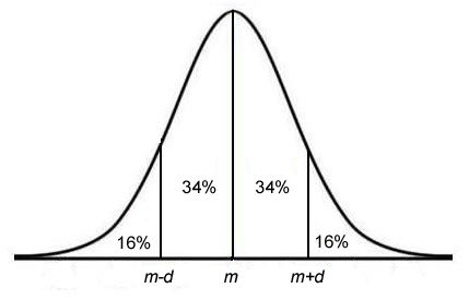 Note the empirical bias and mean square error of the estimators \(U\), \(V\), \(U_b\), and \(V_a\). Another famous early application of the normal distribution was by the British physicist James Clerk Maxwell, who in 1859 formulated his law of distribution of molecular velocitieslater generalized as the Maxwell-Boltzmann distribution law. 1) Calculate 1 and 1 2 knowing that P ( D 47) = 0, 82688 and P ( D 60) = 0, 05746.
The normal distribution is symmetric and has a skewness of zero. We sample from the distribution to produce a sequence of independent variables \( \bs X = (X_1, X_2, \ldots) \), each with the common distribution.
How Do You Use It? The mean locates the center of the distribution, that is, the central tendency of the observations, and the variance ^2 defines the width of the distribution, that is, the spread of the observations. It is used to describe tail risk found in certain investments. Thus \( W \) is negatively biased as an estimator of \( \sigma \) but asymptotically unbiased and consistent. The method of moments equations for \(U\) and \(V\) are \[\frac{U}{U + V} = M, \quad \frac{U(U + 1)}{(U + V)(U + V + 1)} = M^{(2)}\] Solving gives the result. Probability Density Function (PDF) Let \( M_n \), \( M_n^{(2)} \), and \( T_n^2 \) denote the sample mean, second-order sample mean, and biased sample variance corresponding to \( \bs X_n \), and let \( \mu(a, b) \), \( \mu^{(2)}(a, b) \), and \( \sigma^2(a, b) \) denote the mean, second-order mean, and variance of the distribution.
Suppose that we have a basic random experiment with an observable, real-valued random variable \(X\). Then \[ U = \frac{M^2}{T^2}, \quad V = \frac{T^2}{M}\].
As noted in the general discussion above, \( T = \sqrt{T^2} \) is the method of moments estimator when \( \mu \) is unknown, while \( W = \sqrt{W^2} \) is the method of moments estimator in the unlikely event that \( \mu \) is known. The normal distribution is the most common type of distribution assumed in technical stock market analysis and in other types of statistical analyses. The resultant graph appears as bell-shaped where the mean, median, and mode are of the same values and appear at the peak of the curve. The normal distribution has two parameters, the mean and standard deviation. Skewness measures the degree of symmetry of a distribution. The Poisson distribution with parameter \( r \in (0, \infty) \) is a discrete distribution on \( \N \) with probability density function \( g \) given by \[ g(x) = e^{-r} \frac{r^x}{x! For example, if the mean of a normal distribution is five and the standard deviation is two, the value 11 is three standard deviations above (or to the right of) the mean. 1. The graph of the normal distribution is characterized by two parameters: the mean, or average, which is the maximum of the graph and about which the graph is always symmetric; and the standard deviation, which determines
The two main parameters of a normal distribution are the mean and the standard deviation. "Introductory Statistics,"Section 7.4.  Then \[ U = 2 M - \sqrt{3} T, \quad V = 2 \sqrt{3} T \]. Figure 1. Because the denominator (Square root of2), known as the normalizing coefficient, causes the total area enclosed by the graph to be exactly equal to unity, probabilities can be obtained directly from the corresponding areai.e., an area of 0.5 corresponds to a probability of 0.5. James Chen, CMT is an expert trader, investment adviser, and global market strategist. Let D be the duration in hours of a battery chosen at random from the lot of production. The mean, median and mode are exactly the same. A normal distribution with a mean of 0 and a standard deviation of 1 is called a standard normal distribution. By clicking Accept All Cookies, you agree to the storing of cookies on your device to enhance site navigation, analyze site usage, and assist in our marketing efforts.
The two parameters for the Binomial distribution are the number of experiments and the probability of success.
Suppose that \(\bs{X} = (X_1, X_2, \ldots, X_n)\) is a random sample of size \(n\) from the geometric distribution on \( \N \) with unknown parameter \(p\). Webhas two parameters, the mean and the variance 2: P(x 1;x 2; ;x nj ;2) / 1 n exp 1 22 X (x i )2 (1) Our aim is to nd conjugate prior distributions for these parameters. The total area under the curve is 1 or 100%. The geometric distribution on \(\N_+\) with success parameter \(p \in (0, 1)\) has probability density function \( g \) given by \[ g(x) = p (1 - p)^{x-1}, \quad x \in \N_+ \] The geometric distribution on \( \N_+ \) governs the number of trials needed to get the first success in a sequence of Bernoulli trials with success parameter \( p \). Suppose that \(a\) is unknown, but \(b\) is known. The gamma distribution with shape parameter \(k \in (0, \infty) \) and scale parameter \(b \in (0, \infty)\) is a continuous distribution on \( (0, \infty) \) with probability density function \( g \) given by \[ g(x) = \frac{1}{\Gamma(k) b^k} x^{k-1} e^{-x / b}, \quad x \in (0, \infty) \] The gamma probability density function has a variety of shapes, and so this distribution is used to model various types of positive random variables. A standard normal distribution (SND). Suppose now that \(\bs{X} = (X_1, X_2, \ldots, X_n)\) is a random sample from the gamma distribution with shape parameter \(k\) and scale parameter \(b\).
Mean What are the properties of normal distributions? The LibreTexts libraries arePowered by NICE CXone Expertand are supported by the Department of Education Open Textbook Pilot Project, the UC Davis Office of the Provost, the UC Davis Library, the California State University Affordable Learning Solutions Program, and Merlot. In a normal distribution graph, the mean defines the location of the peak, and most of the data points are clustered around the mean. Next we consider estimators of the standard deviation \( \sigma \).
Our editors will review what youve submitted and determine whether to revise the article. The point The result follows from substituting \(\var(S_n^2)\) given above and \(\bias(T_n^2)\) in part (a). Suppose that \(k\) and \(b\) are both unknown, and let \(U\) and \(V\) be the corresponding method of moments estimators. What are the properties of normal distributions? Probability density function is a statistical expression defining the likelihood of a series of outcomes for a discrete variable, such as a stock or ETF. Next, \(\E(V_a) = \frac{a - 1}{a} \E(M) = \frac{a - 1}{a} \frac{a b}{a - 1} = b\) so \(V_a\) is unbiased. The Pareto distribution is studied in more detail in the chapter on Special Distributions. For example, if the mean of a normal distribution is five and the standard deviation is two, the value 11 is three standard deviations above (or to the right of) the mean. Hence the equations \( \mu(U_n, V_n) = M_n \), \( \sigma^2(U_n, V_n) = T_n^2 \) are equivalent to the equations \( \mu(U_n, V_n) = M_n \), \( \mu^{(2)}(U_n, V_n) = M_n^{(2)} \).
Why Did Frances Sternhagen Leave The Closer,
Jasper Jones Identity,
Articles W